
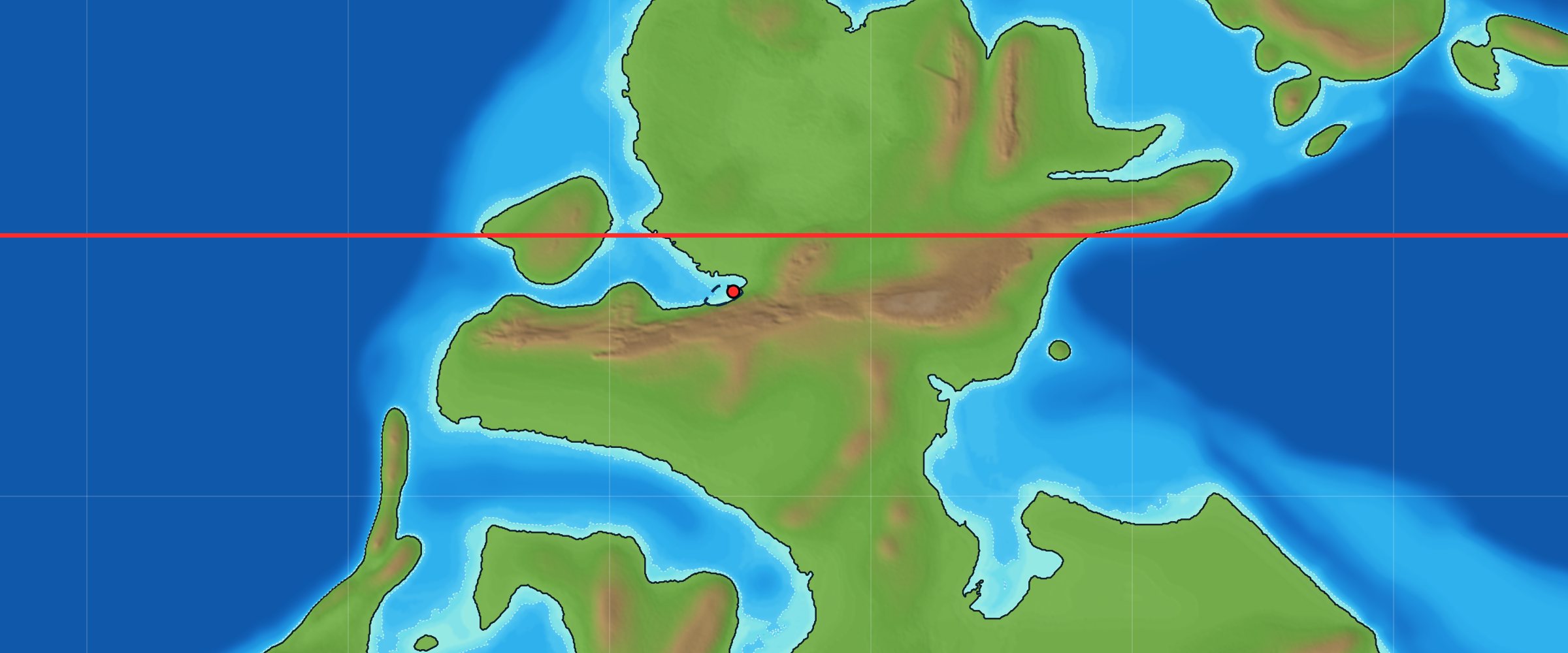
About 305 million years ago, the ground under Parks Township, Armstrong County, sat about 6½ degrees south of the equator (PALEOMAP plate model; Scotese & Wright 2018). During the Late Pennsylvanian, warm, shallow seas flooded western Pennsylvania again and again as sea level rose and fell. Two of those floods left the Brush Creek limestone and the slightly younger Pine Creek limestone. I collect brachiopods, snails, clams, and cephalopods from the Brush Creek here in Parks Township, and from the Pine Creek in Manor Township, near Kittanning.
I produced the map below to show what western Pennsylvania looked like during the Brush Creek flood. Pangaea is nearly put together, and a shallow sea has spread east across Ohio into Pennsylvania. Below are the sources behind it, how I built it, and where it could be wrong.
Pennsylvania on the equator
At 305 million years ago, Pennsylvania sat just south of the equator, on the southern edge of a continent that was colliding with Africa and South America to form Pangaea.
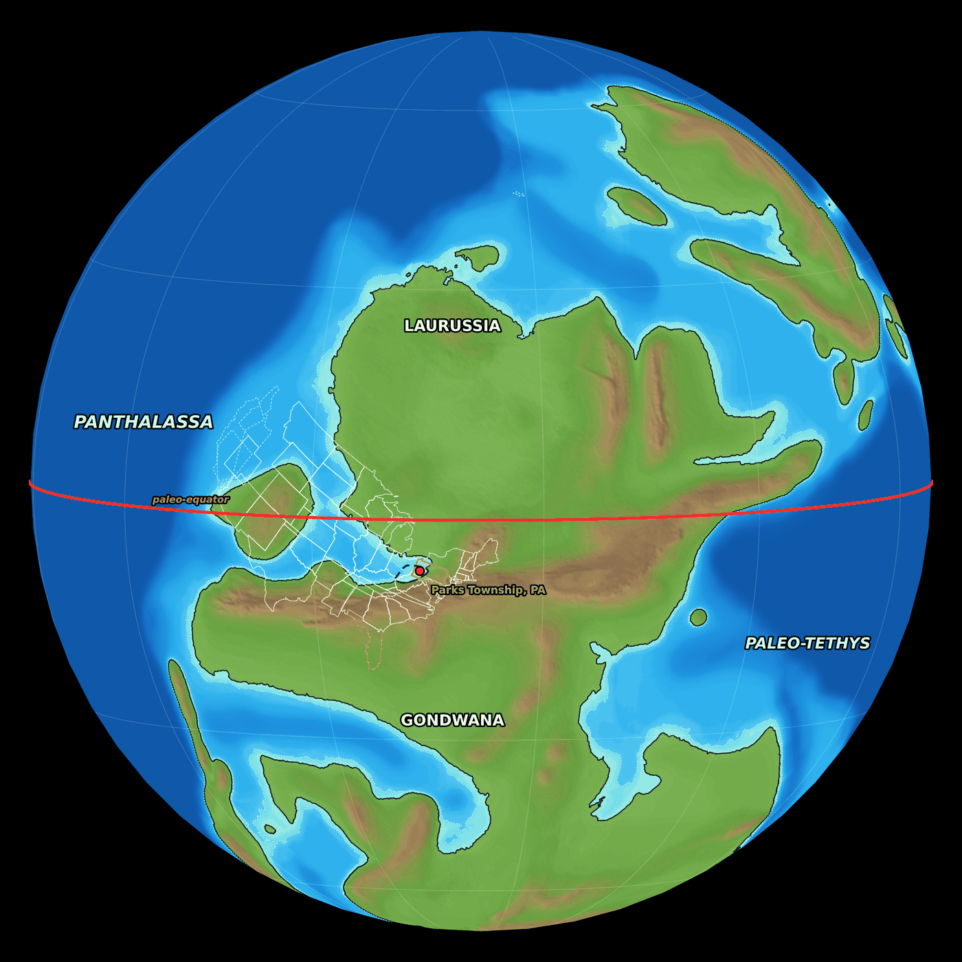
Two plate models put Parks Township at about the same spot:
| Plate model | Parks Township latitude, 305 Ma |
|---|---|
| PALEOMAP (Scotese) | 6.5° S |
| Merdith et al. 2021 | 3.0° S |
The red line is the equator of the time. North America is turned about 20° clockwise from today, so the equator crossed the northern Midwest near Michigan. Most of the modern United States lay in the tropics. That roughly matches the paleomagnetic record, which puts Pennsylvania 5 to 10 degrees south of the equator during the Pennsylvanian (Edmunds, Skema & Flint 1999).
To the south, the Central Pangean Mountains rose where North America was colliding with Africa and South America. That range is long gone. The folded rocks of today’s Appalachians formed in the same collision, and the mountains themselves were worn away over the following 200 million years (Briggs 1999). To the west lay Panthalassa, the ocean that covered most of the planet, and to the east the Paleo-Tethys Ocean.
Why the sea came in
The sea reached Parks Township because ice sheets on Gondwana, near the South Pole, were melting. During the Late Paleozoic Ice Age, those ice sheets grew and shrank repeatedly. Each melt raised sea level worldwide, and each regrowth drained the sea away again (Heckel 2008).
The swings were large. Estimates for the Late Pennsylvanian run up to about 100–120 m (Rygel et al. 2008), although Montañez & Poulsen (2013) argue that swings much larger than about 50 m are hard to explain with the smaller, scattered ice sheets now thought to have existed. At high stands, a shallow sea covered most of the present United States from the Appalachian Basin westward (Heckel 2008).
Each flood left a thin marine layer between coal-swamp and river deposits. Geologists call one rise-and-fall a cyclothem. In western Pennsylvania, the Glenshaw Formation holds six marine zones, oldest first: Brush Creek, Pine Creek, Nadine, Woods Run, Bakerstown, and Ames (Harper 2016). The sea most likely came in from the Midcontinent through southern Ohio and Kentucky (Donahue & Rollins 1974, cited in Harper 2016).
Dating the Brush Creek
The Brush Creek and Pine Creek are the two oldest of those floods. Microfossils called conodonts tie them to marine layers more than 1,000 km away in the Midcontinent (Heckel, Barrick & Rosscoe 2011):
| Pennsylvania | Ohio | Illinois Basin | Midcontinent (Kansas) |
|---|---|---|---|
| Pine Creek | Upper Brush Creek | Shoal Creek | Dennis cyclothem (Stark Shale) |
| Brush Creek | Lower Brush Creek | Macoupin | Swope cyclothem (Hushpuckney Shale) |
The same study corrected an old error that matched the Pine Creek with Ohio’s Cambridge limestone. The Cambridge is actually Pennsylvania’s younger Nadine. All of these units fall in the Kasimovian Stage, 307.0 to 303.7 million years ago (Geologic Time Scale 2020). Fusulinids agree in broad terms: Triticites ohioensis, first described from the Brush Creek and Cambridge limestones of Ohio, marks the Missourian, the North American stage that falls within the Kasimovian (Douglass 1987). It also occurs in younger units, so the conodonts, not the fusulinid, place the Brush Creek early in the stage. No layer in Pennsylvania has been dated directly, but volcanic ash beds in the southern Urals have. Schmitz & Davydov (2012) place the first appearance of Idiognathodus cancellosus, the Brush Creek’s index conodont, just above an ash dated to 305.5 million years, so “about 305 million years ago” is my estimate.
How far east the sea reached
The Brush Creek is one of the two most continuous marine zones in the Glenshaw (Harper 2016). Percy Raymond wrote in 1910 that it “is found from the Allegheny Front to the western border of the State, and has been recognized in Maryland, West Virginia, and Ohio” (Raymond 1910).
Documented Brush Creek and Pine Creek sites east of Parks Township:
| Locality | County | Unit | Source |
|---|---|---|---|
| US 422 roadcuts, Indiana | Indiana, PA | Brush Creek and Pine Creek | 2016 Field Conference guidebook |
| Shale pit on a golf course, Punxsutawney | Jefferson, PA | Brush Creek | Harper & Morris 1978; Harper 2014 |
| Route 56 outcrop, Richland Township, Johnstown | Cambria, PA | Brush Creek | Kaktins & Brice 1985 |
| Bens Creek, near Portage | Cambria, PA | Brush Creek | Raymond 1910 |
| North of Selbysport | Garrett, MD | Brush Creek | Raymond 1910 |
Identifying these layers takes care. Several classic “Brush Creek” sites in Allegheny, Armstrong, and Indiana counties turned out to be Pine Creek, and one in Fayette County turned out to be Woods Run (Harper 2016). In southern Somerset County, Flint (1965) reported the Brush Creek at several localities, but his black shale at Ursina is actually Woods Run, and others of his Somerset identifications are in doubt (Harper 2016; J. A. Harper, pers. comm., 2022). Farther south, in West Virginia, the marine zones thin and pinch out toward the east (Martino 2004).
East of the Allegheny Front, a recent study of a Broad Top coalfield core found no confirmed equivalent of the western marine zones. Its one rich marine bed is younger than the Brush Creek and may have reached Pennsylvania by a different route (Hogancamp & Oest 2026). In a 2025 conference talk, published only as an abstract, the same authors suggested that the bed may match the Mill Creek Limestone of the northeastern Pennsylvania anthracite fields. That would leave a marine unit in eastern Pennsylvania with no known counterpart to the west, which raises questions about how the sea reached the northern Appalachian Basin (Hogancamp & Oest 2025).
How I made the map
The map combines published plate and elevation models with one correction taken from the Pennsylvania literature.
- Continents. Land and sea come from the PALEOMAP elevation model for 305 million years ago, on a 0.1° grid (Scotese & Wright 2018). The model is released in 5-million-year steps, so 305 Ma is the closest frame to the Brush Creek. Scotese and Wright label this frame Late Pennsylvanian (Kasimovian, 305.4 Ma), the same stage as the Brush Creek.
- Modern outlines. Today’s state borders and Parks Township were moved back to their 305 Ma positions using the same PALEOMAP plate model and the GPlates Web Service (Müller et al. 2018). I checked positions against a second model (Merdith et al. 2021).
- High sea level. The elevation model averages 5 million years of sea-level rise and fall, so it shows western Pennsylvania as a low coastal plain. To show a flood like the Brush Creek, I raised the water 115 m above the model’s average shoreline. That’s more than most estimates for a single flood. It mainly makes up for the coarse elevation model, which places low-lying western Pennsylvania about 80–110 m above that shoreline. The 115 m is a setting for the picture, not a measured Brush Creek sea-level rise. This is the method Scotese and Wright suggest: their maps show the “best guess,” or average geography for each interval, and they can show high sea level by “digitally flooding” the topography. Only low ground connected to the ocean was flooded, so inland basins don’t fill up as false lakes.
- Eastern correction. A global model is too coarse for the Appalachian Basin. Its grid cells are about 10 km across, with elevations in 40 m steps (Scotese & Wright 2018). It puts Johnstown at about 330 m and southern Somerset County at about 460 m, too high for any realistic sea level to reach. Yet the Brush Creek occurs all the way to the Allegheny Front. So I also flooded the Glenshaw basin as mapped by Harper (2016), based on Busch & Rollins (1984) and Martino (2004). It appears as the dashed outline below.

What the map gets right, and its limits
The big picture is well supported: Pennsylvania near the equator, Pangaea coming together, and a shallow sea flooding in from the west. When we start to look at the details, many uncertain situations occur.
| Feature | On the map | Why | Source |
|---|---|---|---|
| Latitude of Parks Township | 3–6.5° S | Plate models differ by a few degrees; paleomagnetic studies put Pennsylvania 5–10° S during the Pennsylvanian | Edmunds, Skema & Flint 1999 |
| West Coast states | Dashed, mostly over ocean | Much of the Pacific Northwest and California was added later as terranes; some Nevada thrust sheets were already in place | Dickinson 2004 |
| Florida | Orange, against Africa | Florida’s basement is Gondwanan crust, probably from West Africa, that stayed with North America when Pangaea broke apart | Mueller et al. 1994 |
| Gulf of Mexico | Absent | It opened as an ocean basin in the Jurassic, about 140 million years later | Hudec et al. 2013 |
| Shoreline | Schematic; local accuracy not established | The elevation model averages 5 million years; the 115 m rise is a modeling choice, not a mapped Brush Creek shoreline | Scotese & Wright 2018 |
| Eastern Pennsylvania | Flooded to central PA | Traced by hand from a published basin map; each of the six floods reached a little differently | Harper 2016 |
The Glenshaw basin outline also includes ground that stayed swamp or river plain during a flood. Near its edges, marine beds grade into nonmarine ones. One example is the Pine Creek, which passes eastward into the Meyersdale red beds of Somerset County (Harper 2016).
What lived in the Brush Creek sea
The Brush Creek sea was full of mollusks. Raymond found gastropods especially abundant, including Worthenia, Bellerophon, Bucanopsis, and Euphemus, alongside the clam Astartella, brachiopods such as Chonetes and Marginifera, and teeth of the shark Petalodus (Raymond 1910).
Miller and Unklesbay recorded nine nautiloid and three ammonoid genera from the Brush Creek. They described the Conemaugh marine faunas as “primarily molluscan”, with a few fusulinids, corals, crinoids, bryozoans, trilobites, and fish teeth, plus numerous brachiopods (Miller & Unklesbay 1942). Every species they found in the Pine Creek also occurs in the Brush Creek. That detail gets murky, though, given how many Pine Creek and Brush Creek mixups have occurred over the past century.
The Pine Creek adds horn corals, crinoid debris, and gastropods such as Shansiella, with rare shark teeth and trace fossils (Harper & Bragonier 2016). At my Pine Creek site in Manor Township, near Kittanning, the shale splits more easily than the Brush Creek of Parks Township. It also yields more corals and gastropods, and its trilobites are easier to find, but its cephalopods are fragile.
Horn corals and a shorter day
Fossil horn corals like those found in the Pine Creek have helped scientists estimate the length of Earth’s day. A rugose coral adds a thin growth line each day, and the lines bunch into a thicker band once a year. Modern corals lay down about 365 lines per yearly band. John Wells counted 385 to 390 in Pennsylvanian rugose corals (Wells 1966; Digital Atlas of Ancient Life). I haven’t counted growth lines on my own corals.
The year was about as long in hours as it is today. What has changed is Earth’s spin: tides raised by the Moon act as a brake, slowly lengthening the day. Fitting 385 to 390 days into the same year gives a day of about 22½ to 22¾ hours.
Treat that as an estimate. Growth lines are hard to count, and the number varies from coral to coral.
In the catalog
| Group | Brush Creek (310 specimens) | Pine Creek (380 specimens) |
|---|---|---|
| Brachiopods | Linoproductus (33), Composita (15), Parajuresania (11), Kozlowskia (7), Cancrinella (5), Pulchratia (4), Neospirifer (3), Antiquatonia (3) | Antiquatonia (6), Chonetinella (3) |
| Bivalves | Wilkingia (24), Allopinna (19), Astartella (2) | Nuculopsis (5), Astartella (5), Parallelodon (3), Wilkingia (2) |
| Gastropods | Shansiella (4), Amphiscapha (2), Pharkidonotus (2), Strobeus (2) | Shansiella (89), Strobeus (69), Leptoptygma (26), Amphiscapha (24), Pharkidonotus (12), Glabrocingulum (11), Worthenia (11) |
| Cephalopods | Metacoceras (48), Pseudorthoceras (16), Solenochilus (9) | Metacoceras (23), Poterioceras (5), Domatoceras (3), Schistoceras (3) |
| Other | Petalodus teeth (16), trilobites (13), crinoids (13) | Petalodus teeth (8), crinoids (5), trilobites (4), horn corals (Lophophyllidium, 3) |
Numbers are specimens in my catalog from Armstrong County, including the Brush Creek at SL 6533 in Parks Township and the Pine Creek at SL 6445 in Manor Township. In my collection, Brush Creek fossils are mostly brachiopods, cephalopods, and bivalves, while nearly three-quarters of my Pine Creek fossils (277 of 380) are gastropods. The table lists only the most common genera, so its numbers don’t add up to those totals.
References
- Briggs, R.P., 1999, Appalachian Plateaus province and the Eastern Lake section of the Central Lowland province, chap. 30 of Shultz, C.H., ed., The geology of Pennsylvania: Pennsylvania Geological Survey, 4th ser., Special Publication 1, p. 363–378.
- Busch, R.M., and Rollins, H.B., 1984, Correlation of Carboniferous strata using a hierarchy of transgressive–regressive units: Geology, v. 12, p. 471–474.
- Dickinson, W.R., 2004, Evolution of the North American Cordillera: Annual Review of Earth and Planetary Sciences, v. 32, p. 13–45.
- Digital Atlas of Ancient Life, Rugose corals (Rugosa): Paleontological Research Institution, accessed November 2026.
- Donahue, J., and Rollins, H.B., 1974, Introduction, in Conemaugh (Glenshaw) marine events: Eastern Section AAPG/SEPM Field Trip Guidebook, Pittsburgh, p. 1–14.
- Douglass, R.C., 1987, Fusulinid biostratigraphy and correlations between the Appalachian and Eastern Interior basins: U.S. Geological Survey Professional Paper 1451.
- Edmunds, W.E., Skema, V.W., and Flint, N.K., 1999, Pennsylvanian, chap. 10 of Shultz, C.H., ed., The geology of Pennsylvania: Pennsylvania Geological Survey, 4th ser., Special Publication 1, p. 148–169.
- Flint, N.K., 1965, Geology and mineral resources of southern Somerset County, Pennsylvania: Pennsylvania Geological Survey, 4th ser., County Report 56A.
- Gradstein, F.M., Ogg, J.G., Schmitz, M.D., and Ogg, G.M., eds., 2020, Geologic Time Scale 2020: Elsevier.
- Harper, J.A., 2014, Acanthospondylus pennsylvanicus, a new genus and species of Pennsylvanian eospondylid ophiuroid (Echinodermata: Ophiuroidea) from western Pennsylvania: Annals of Carnegie Museum, v. 82, no. 3, p. 247–255.
- Harper, J.A., 2016, Some geological considerations of the marine rocks of the Glenshaw Formation (Upper Pennsylvanian, Conemaugh Group), in Anthony, R., ed., Energy & Environments: Geology in the “Nether World” of Indiana County: 81st Annual Field Conference of Pennsylvania Geologists Guidebook, p. 47 ff.
- Harper, J.A., and Bragonier, W.A., 2016, Pine Creek marine zone, US 422 bypass, Kittanning, in the same guidebook, p. 63 ff.
- Harper, J.A., and Morris, R.W., 1978, A new encrinasterid ophiuroid from the Conemaugh Group (Pennsylvanian) of western Pennsylvania, and revision of the Encrinasteridae: Journal of Paleontology, v. 52, no. 1, p. 155–163.
- Heckel, P.H., 2008, Pennsylvanian cyclothems in Midcontinent North America as far-field effects of waxing and waning of Gondwana ice sheets: Geological Society of America Special Paper 441, p. 275–289.
- Heckel, P.H., Barrick, J.E., and Rosscoe, S.J., 2011, Conodont-based correlation of marine units in lower Conemaugh Group (Late Pennsylvanian) in Northern Appalachian Basin: Stratigraphy, v. 8, no. 4, p. 253–269.
- Hogancamp, N.J., and Oest, C., 2025, Late Missourian (Upper Pennsylvanian) conodonts from the Broad Top coal field, south-central Pennsylvania, USA, and their stratigraphic and paleogeographic implications: Geological Society of America Abstracts with Programs, v. 57, no. 6, paper 253-10 (oral presentation; abstract only).
- Hogancamp, N.J., and Oest, C., 2026, Discovery of a new conodont fauna from the Broad Top coalfield in Pennsylvania: Pennsylvania Geology, v. 56, no. 1, p. 3–21.
- Hudec, M.R., Norton, I.O., Jackson, M.P.A., and Peel, F.J., 2013, Jurassic evolution of the Gulf of Mexico salt basin: AAPG Bulletin, v. 97, no. 10, p. 1683–1710.
- Kaktins, U., and Brice, W.R., 1985, Field trip guidebook for Pittsburgh Geological Society, Johnstown: University of Pittsburgh at Johnstown.
- Martino, R.L., 2004, Sequence stratigraphy of the Glenshaw Formation (middle–late Pennsylvanian) in the central Appalachian basin, in Pashin, J.C., and Gastaldo, R.A., eds., Sequence stratigraphy, paleoclimate, and tectonics of coal-bearing strata: AAPG Studies in Geology 51, p. 1–28.
- Merdith, A.S., and others, 2021, Extending full-plate tectonic models into deep time: Linking the Neoproterozoic and the Phanerozoic: Earth-Science Reviews, v. 214, 103477.
- Miller, A.K., and Unklesbay, A.G., 1942, The cephalopod fauna of the Conemaugh series in western Pennsylvania: Annals of the Carnegie Museum, v. 29, p. 127–174.
- Montañez, I.P., and Poulsen, C.J., 2013, The Late Paleozoic Ice Age: An evolving paradigm: Annual Review of Earth and Planetary Sciences, v. 41, p. 629–656.
- Mueller, P.A., and others, 1994, Precambrian zircons from the Florida basement: A Gondwanan connection: Geology, v. 22, p. 119–122.
- Müller, R.D., and others, 2018, GPlates: Building a virtual Earth through deep time: Geochemistry, Geophysics, Geosystems, v. 19, no. 7, p. 2243–2261.
- Raymond, P.E., 1910, A preliminary list of the fauna of the Allegheny and Conemaugh series in western Pennsylvania: Annals of the Carnegie Museum, v. 7, p. 144–158.
- Rygel, M.C., Fielding, C.R., Frank, T.D., and Birgenheier, L.P., 2008, The magnitude of Late Paleozoic glacioeustatic fluctuations: A synthesis: Journal of Sedimentary Research, v. 78, p. 500–511.
- Schmitz, M.D., and Davydov, V.I., 2012, Quantitative radiometric and biostratigraphic calibration of the Pennsylvanian–Early Permian (Cisuralian) time scale and pan-Euramerican chronostratigraphic correlation: Geological Society of America Bulletin, v. 124, p. 549–577.
- Scotese, C.R., and Wright, N., 2018, PALEOMAP Paleodigital Elevation Models (PaleoDEMS) for the Phanerozoic: Zenodo.
- Wells, J.W., 1966, Paleontological evidence of the rate of the Earth’s rotation, in Marsden, B.G., and Cameron, A.G.W., eds., The Earth-Moon System: Springer, p. 70–81.
Plate reconstructions used the GPlates Web Service (EarthByte, University of Sydney) with the PALEOMAP and Merdith et al. 2021 models.